Additional Features
ChemPlot offers additional features for chemical space visualization which can improve the understanding of the underlying similarities between the investigated molecules.
Using the Plotter object it is possible to create two different kind plots of
the chemical space, aside from the scatterplots showed in the previous sections.
These plots investigate the density distribution of the chemical space an are
hexagonal bin plot and the kernel density estimate plot.
To show the before mentioned features we will use the BBBP (blood-brain barrier penetration) dataset [1], already mentioned in the previous section:
from chemplot import Plotter, load_data

data_BBBP = load_data("BBBP")
cp_BBBP = Plotter.from_smiles(data_BBBP["smiles"], target=data_BBBP["target"], target_type="C")
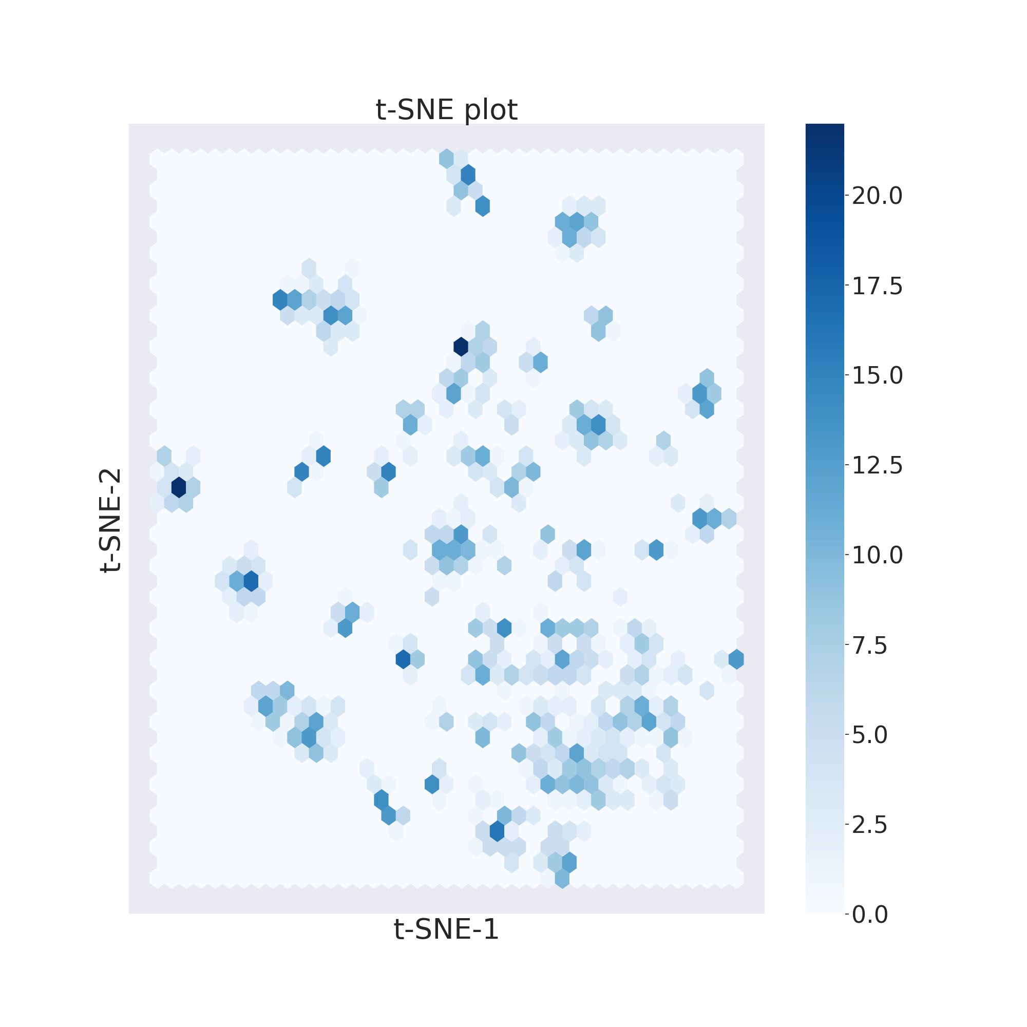
Hexagonal Bin Plot
In a hexagonal bin plot points are binned into hexagons, which in turn are
coloured depending on the count of observations they cover. To create a
hexagonal bin plot we need to pass the keyword “hex” as the kind
parameter when visualizing the plot.
cp_BBBP.tsne(random_state=0)
cp_BBBP.visualize_plot(kind="hex")
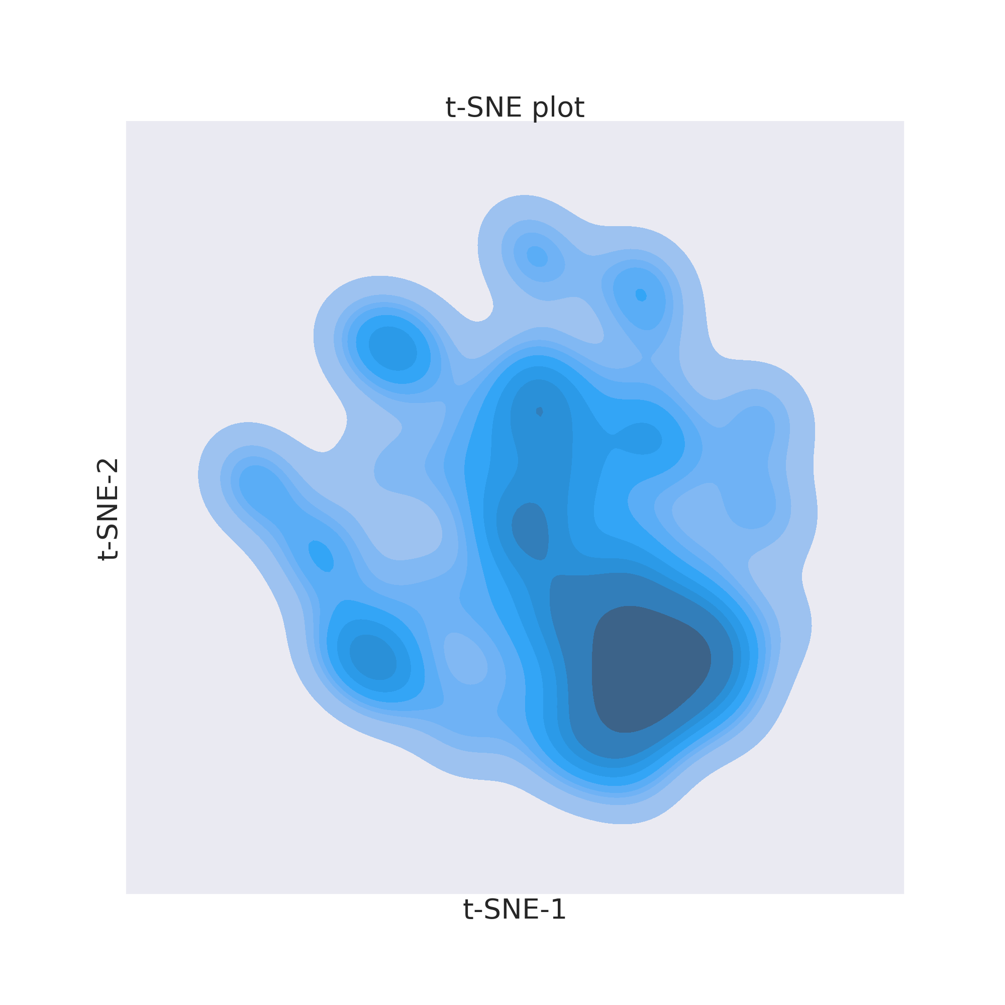
Kernel Density Estimate Plot
In a kernel density estimate plot, the data distribution is visualized by a
continuous probability density curve which in our case is in 2 dimensions. To
create a kernel density estimate plot we need to pass the keyword “kde” as the
kind parameter when visualizing the plot.
cp_BBBP.visualize_plot(kind="kde")
References: