How to use ChemPlot

ChemPlot is a cheminformatics tool whose purpose is to visualize subsets of the chemical space in two dimensions. It uses the RDKit chemistry framework, the scikit-learn API and the umap-learn API.

Getting started

To demonstrate how to use the functions the library offers we will use a BBBP (blood-brain barrier penetration) 1 molecular dataset. This is a set of molecules encoded as SMILES, which have been assigned a binary label according to their permeability properties. This dataset can be loaded as a pandas <https://pandas.pydata.org/pandas-docs/stable/index.html>`_ DataFrame object.

from pandas import read_csv

data_BBBP = read_csv("BBBP.csv")

To visualize the molecules in 2D according to their similarity it is first needed to construct a Plotter object. This is the class containing all the functions ChemPlot uses to produce the desired visualizations. A Plotter object can be constructed using classmethods, which differentiate between the type of input that is feed to the object. In our example we need to use the method from_smiles. We pass three parameters: the list of SMILES from the BBBP dataset, their target values (the binary labels) and the target type (in this case “C”, which stands for “Classification”).

from chemplot import Plotter

cp = Plotter.from_smiles(data_BBBP["smiles"], target=data_BBBP["target"], target_type="C")

Plotting the results

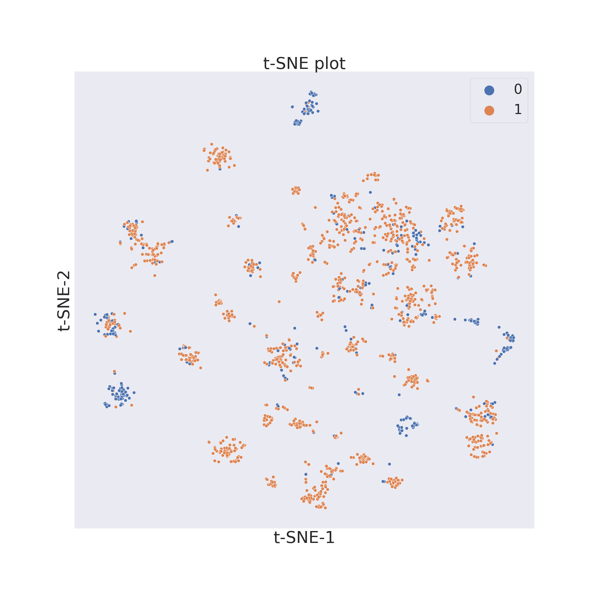
When the Plotter object was constructed, descriptors for each SMILES were calculated, using the library mordred, and then selected based on the target values. We reduce the number of dimensions for each molecule from the number of descriptors selected to only 2. ChemPlot uses three different algorithms in order to achieve this. In this example we will first use t-SNE 2.

cp.tsne()

The output will be a dataframe containg the reduced dimensions and the target values.

t-SNE-1	t-SNE-2	target
-41.056122	0.355575	1
-35.535915	21.648867	1
23.771597	-14.438373	1

To now visualize the chemical space of the dataset we use visualize_plot().

import matplotlib.pyplot as plt

cp.visualize_plot()

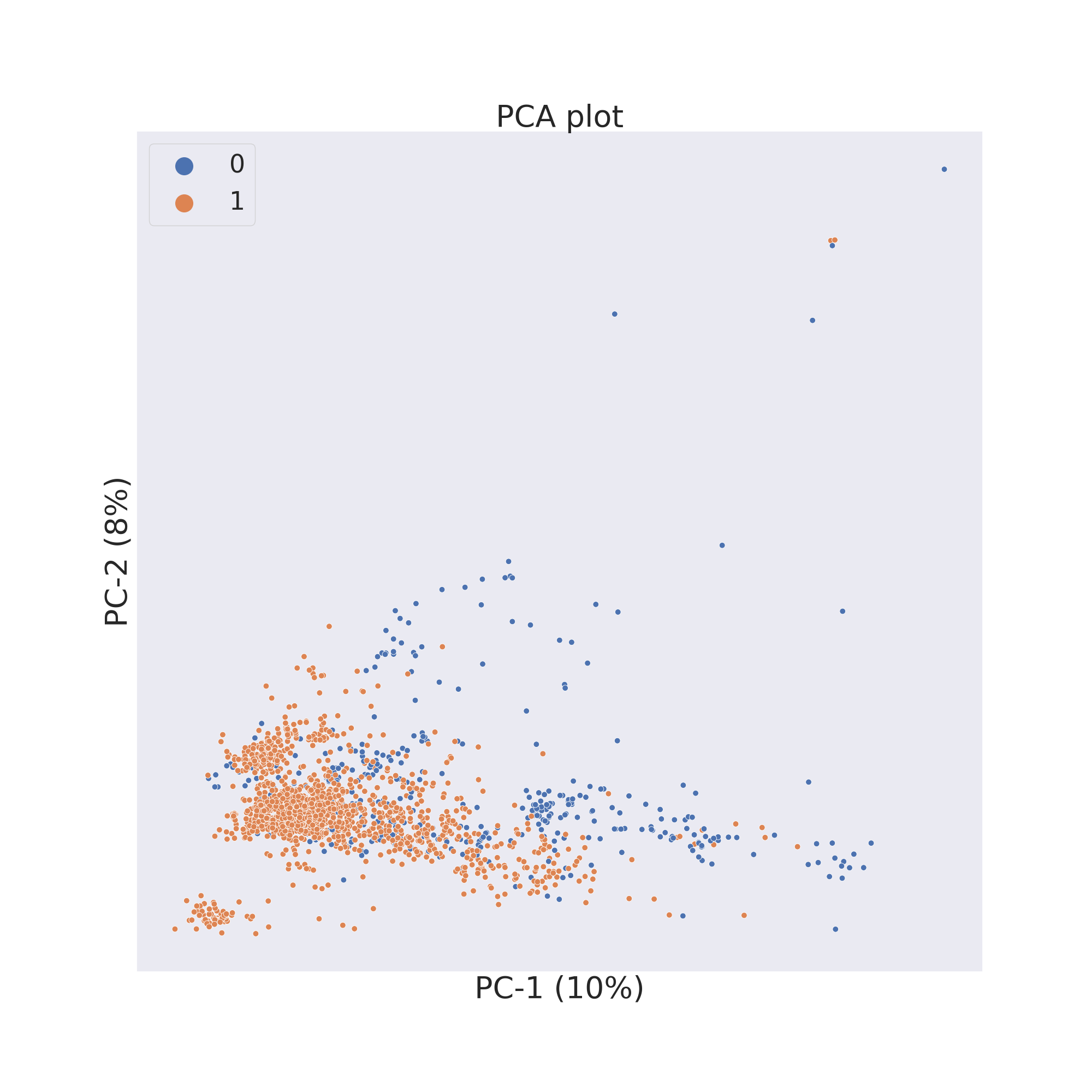
The second figure shows the results obtained by reducing the dimensions of features Principal Component Analysis (PCA) 3.

cp.pca()
cp.visualize_plot()

The third figure shows the results obtained by reducing the dimensions of features by UMAP 4.

cp.umap()
cp.visualize_plot()

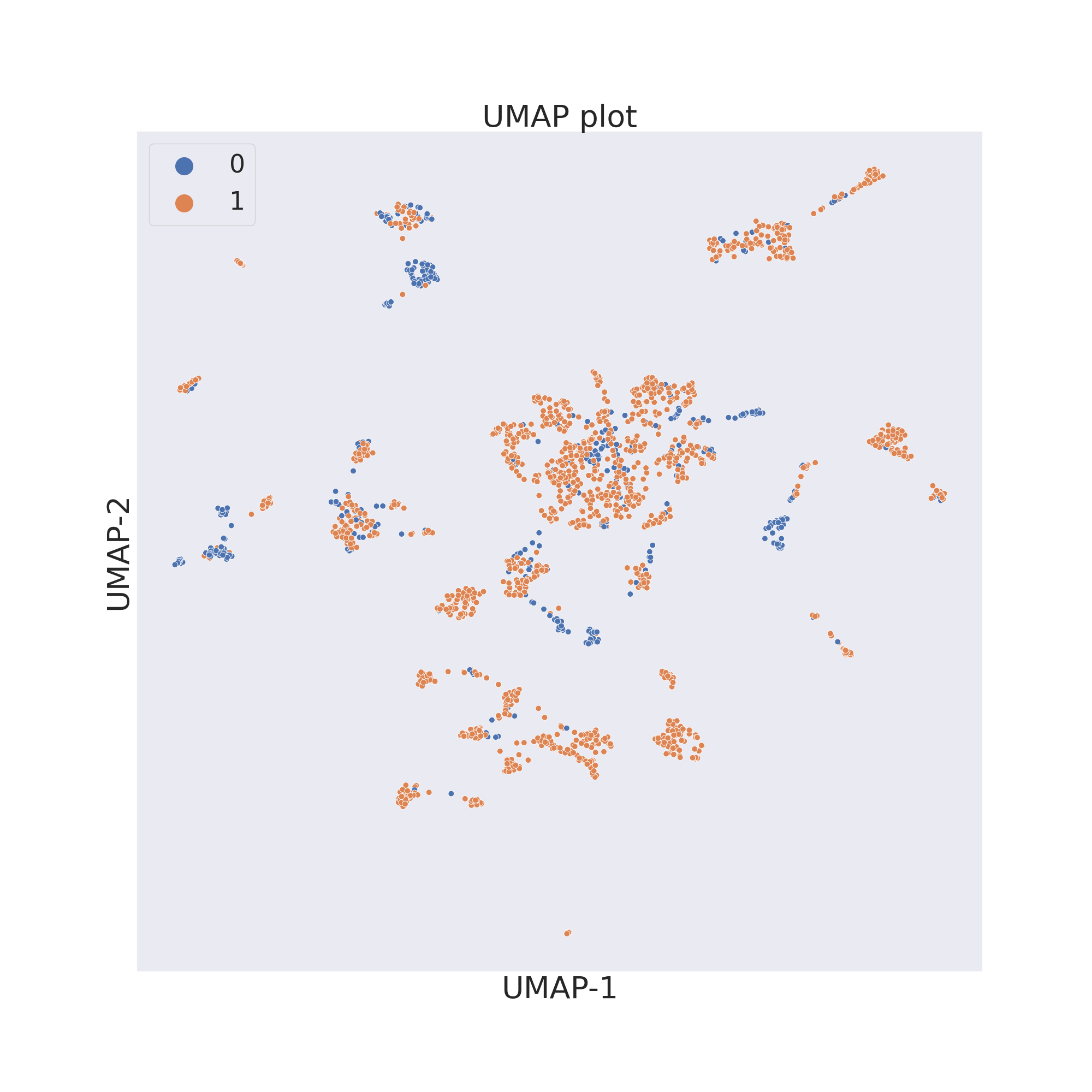
In each figure the molecules are coloured by class value.

---

References:

1

Martins, Ines Filipa, et al. (2012). A Bayesian approach to in silico blood-brain barrier penetration modeling. Journal of chemical information and modeling 52.6, 1686-1697

2

van der Maaten, Laurens, Hinton, Geoffrey. (2008). Viualizingdata using t-SNE. Journal of Machine Learning Research. 9. 2579-2605.

3

Wold, S., Esbensen, K., Geladi, P. (1987). Principal component analysis. Chemometrics and intelligent laboratory systems. 2(1-3). 37-52.

4

McInnes, L., Healy, J., Melville, J. (2018). Umap: Uniform manifold approximation and projection for dimension reduction. arXivpreprint arXiv:1802.03426.